Numerical schemes generated by Bezier splines
I consider ordinary differential equations of the form
\[\mathbf{\dot y}(t) = f(\mathbf{y},t) = \mathbf{A y}(t)\]I will show how the bezier splines lead naturally to well known numerical integration schemes while giving a meaningful interpretation to their intermediate control points in term of forward-backward taylor series prediction.
This class of methods belong to the class of multi-derivative integrators and are known as Hermite-Obreshkoff. While much less known than the Runge-Kutta methods, they can also regenerate the Padé approximations of the exponential map while providing piece-wise \(C^k\) continuous trajectory approximations.
In the following, to simplify notation, each time step is normalised to \([0,1]\) thus the \(A\) matrix is supposed to be pre-normalised by the stepsize \(h\)
In the general case a Bezier Spline is defined by
\[\mathbf B(t) = \sum_{k=0}^{n} \mathbf P_k B_k^n(t)\]For the control points \(\{ \mathbf P_k \}\) and the Bernstein polynomial basis functions
\[B_k^n(t) = \binom{n}{k} (1-t)^{n-k} t^k\]with \(\binom{n}{k}\) being the binomial coefficients.
We will first study the well-known Linear, Quadratic and Cubic bezier splines and the respective numerical schemes that they can generate.
Linear Bezier spline
The linear bezier spline is defined for \(t \in [0,1]\) and the control points \(\mathbf{P_0, P_1} \in \mathbb{R}^d\) as
\[\begin{align} \mathbf{B}(t) &= \mathbf{P_0}(1-t) + \mathbf{P_1} t \\ \label{LinearBezierDerivative} \mathbf{\dot B}(t) &= \mathbf{P_1 - P_0} \end{align}\]where \(\mathbf{P_0, P_1}\) are the end-points of the curve.
By evaluating The above equations for \(t=\left\{0, \frac{1}{2}, 1\right\}\) we get the following relations:
\[\begin{align} \mathbf{P_1 - P_0} &= A \mathbf{P_0} \\ \mathbf{P_1 - P_0} &= A \left(\frac{\mathbf{P_1 + P_0}}{2}\right) \\ \mathbf{P_1 - P_0} &= A \mathbf{P_1} \end{align}\]By combining these equations, we can generate several different approximations that we will label \((m,n)\) according to the fact that we use order \(m\) forward prediction and order \(n\) backward prediction.
Forward Euler (1,0)
Using the first relation and solving for \(P_1\) leads to the following forward prediction:
\[\mathbf{P_1} = (I+A) \mathbf{P_0}\]with stability region
\[R(z) = 1+z\]Remark: this is the Pade (1,0) approximation of \(e^z\)
Mid-point
Using the second relation and solving for \(P_1\) leads to the following prediction:
\[\mathbf{P_1} = \left(I-\frac{A}{2}\right)^{-1} \left(I+\frac{A}{2}\right) \mathbf{P_0}\]with stability region
\[R(z) = \frac{1+\frac{z}{2}}{1-\frac{z}{2}}\]Remark: This is the Pade (1,1) approximation of \(e^z\). The symmetry of the collocation point within the interval allows to reach a consistency of order 2 while the polynomial is only of degree 1.
Backward Euler (0,1)
Using The third equation and solving for \(P_1\) leads to the following prediction:
\[\mathbf{P_1} = (I-A)^{-1} \mathbf{P_0}\]with stability region
\[R(z) = \frac{1}{1-z}\]Remark: This is the Pade (0,1) approximation of \(e^z\)
Quadratic Bezier Spline
The quadratic bezier spline is defined for \(t \in [0,1]\) and the control points \(\mathbf{P_0, P_1, P_2} \in \mathbb{R}^d\) as
\[\begin{align} \mathbf{B}(t) &= \mathbf{P_0}(1-t)^2 + \mathbf{P_1} 2(1-t)t + \mathbf{P_2} t^2 \\ \label{QuadraticBezierDerivative} \mathbf{\dot B}(t) &= 2(1-t)\mathbf{(P_1 - P_0)} + 2t \mathbf{(P_2 - P_1)} \\ \label{QuadraticBezierSecondDerivative} \mathbf{\ddot B}(t) &= 2\mathbf{(P_2 - 2P_1 + P_0)} \end{align}\]where \(\mathbf{P_0, P_2}\) are the end-points of the curve and \(\mathbf{P_1}\) is a control point not belonging to the curve but having an effect on its derivative.
When integrating an ODE we only know \(\mathbf{P_0}\) so we need a way to estimate \(\mathbf{P_1, P_2}\). For this several choices are possible.
By evaluating the first derivative for \(t \in \{0,1\}\) we get the following relations:
\[\begin{align} \label{QuadForward} \mathbf{P_1} &= \left(I+\frac{A}{2}\right)\mathbf{P_0} \\ \label{QuadBackward} \mathbf{P_1} &= \left(I-\frac{A}{2}\right)\mathbf{P_2} \end{align}\]\(\mathbf{P_1}\) can be interpreted both as the truncated forward taylor series prediction of order 1 from \(t=0 \to \frac{1}{2}\) and as the truncated backward taylor series prediction of order 1 from \(t=1 \to \frac{1}{2}\)
And by evaluating the second derivative for \(t \in \{0,1\}\) we get the following relations:
\[\begin{align} \label{QuadForward2} \mathbf{P_2} = \left(I + A + \frac{A^2}{2}\right)\mathbf{P_0}\\ \label{QuadBackward2} \mathbf{P_0} = \left(I - A + \frac{A^2}{2}\right)\mathbf{P_2} \end{align}\]which are respectively the truncated forward taylor series prediction of order 2 from \(t=0 \to 1\) and as the truncated backward taylor series prediction of order 1 from \(t=1 \to 0\)
By combining these 4 equations we can generate several different approximations that we will label \((m,n)\) according to the fact that we use order \(m\) forward prediction and order \(n\) backward prediction.
As we have demonstrated in the previous section, this is equivalent to matching respectively the first $m,n$ derivatives of the exact solution on the left and right of the interval.
Quadratic (2,0)
Using forward predictions leads to the following equations:
\[\begin{align} \mathbf{P_1} &= \left(I+\frac{A}{2}\right) \mathbf{P_0} \\ \mathbf{P_2} &= \left(I+A+\frac{A^2}{2}\right) \mathbf{P_0} \end{align}\]with stability region
\[R(z) = 1+z+\frac{z^2}{2}\]Remark: This is the Pade (2,0) approximation of \(e^z\).
Quadratic (1,1)
Using Forward-Backward equations leads to the following prediction, which is equivalent to the bilinear method / trapezoidal rule:
\[\begin{align} \mathbf{P_1} &= \left(I+\frac{A}{2}\right) \mathbf{P_0} \\ \mathbf{P_2} &= \left(I-\frac{A}{2}\right)^{-1}\mathbf{P_1} = \left(I-\frac{A}{2}\right)^{-1}\left(I+\frac{A}{2}\right) \mathbf{P_0} \end{align}\]with stability region
\[R(z) = \frac{1+\frac{z}{2}}{1-\frac{z}{2}}\]Remark: This is the Pade (1,1) approximation of \(e^z\).
Quadratic (0,2)
Using first and second order backward predictions leads to the following equations:
\[\begin{align} \mathbf{P_1} &= \left(I-\frac{A}{2}\right) \mathbf{P_2} \\ \mathbf{P_2} &= \left(I-A+\frac{A^2}{2}\right)^{-1}\mathbf{P_0} \end{align}\]with stability region
\[R(z) = \frac{1}{1-z+\frac{z^2}{2}}\]Remark: This is the Pade (0,2) approximation of \(e^z\).
Cubic Bezier Spline
The cubic bezier spline is defined for \(t \in [0,1]\) and the control points \(\mathbf{P_0, P_1, P_2, P_3} \in \mathbb{R}^d\) as
\[\begin{align} \mathbf{B}(t) &= \mathbf{P_0}(1-t)^3 + \mathbf{P_1} 3(1-t)^2t + \mathbf{P_2} 3(1-t)t^2 + \mathbf{P_3}t^3\\ \label{CubicBezierDerivative} \mathbf{\dot B}(t) &= 3(1-t)^2\mathbf{(P_1 - P_0)} + 6(1-t)t \mathbf{(P_2 - P_1)} + 3t^2 \mathbf{(P_3 - P_2)}\\ \label{CubicBezierSecondDerivative} \mathbf{\ddot B}(t) &= 6(1-t)\mathbf{(P_2 - 2P_1 + P_0)} + 6t \mathbf{(P_3 - 2P_2 + P_1)} \\ \label{CubicBezierThirdDerivative} \mathbf{\dddot B}(t) &= 6\mathbf{(P_3 - 3P_2 + 3P_1 - P_0)} \end{align}\]where \(\mathbf{P_0, P_3}\) are the end-points of the curve and \(\mathbf{P_0, P_1 P_2, P_3 }\) is the control polygon.
By evaluating the first, second and third derivative for \(t \in \{0,1\}\) and rearranging terms, we get the following relations:
\[\begin{align} \label{cubicP1} \mathbf{P_1} &= \left(I+\frac{A}{3}\right)\mathbf{P_0} \\ \label{cubicP2} \mathbf{P_2} &= \left(I-\frac{A}{3}\right)\mathbf{P_3} \\ \label{CubicFWD} \mathbf{P_2} &= \left(I + \frac{2}{3}A + \frac{A^2}{6}\right))\mathbf{P_0} \\ \label{CubicBWD} \mathbf{P_1} &= \left(I - \frac{2}{3}A + \frac{A^2}{6}\right))\mathbf{P_3} \\ \label{CubicFWD3} \mathbf{P_3} &= \left(I + A + \frac{A^2}{2} + \frac{A^3}{6}\right))\mathbf{P_0} \\ \label{CubicBWD3} \mathbf{P_0} &= \left(I - A + \frac{A^2}{2} - \frac{A^3}{6}\right))\mathbf{P_3} \end{align}\]These are respectively the forward (backward) taylor series prediction of order \(1,2,3\) from \(0 \to \frac{1}{3}\), \(1 \to \frac{2}{3}\), \(0 \to \frac{2}{3}\), \(1 \to \frac{1}{3}\), \(0 \to 1\), \(1 \to 0\)
While evaluating for \(t=\frac{1}{2}\) gives:
\[\begin{align} \label{CubicMid} \frac{3}{4} \left(\mathbf{P_3 + P_2 - (P_1 + P_0)}\right) = A\left(\frac{\mathbf{P_0 + 3 P_1 + 3 P_2 + P_3}}{8} \right) \end{align}\]Mixing equations leads to different numerical approximations corresponding to the Pade (m,n) approximations of \(e^z\) with \(m+n=3\).
Cubic (3,0)
Choosing forward prediction leads to
\[\begin{align} \mathbf{P_1} &= \left(I + \frac{A}{3}\right)\mathbf{P_0} \\ \mathbf{P_2} &= \left(I+\frac{2A}{3} + \frac{A^2}{6}\right) \mathbf{P_0} \\ \mathbf{P_3} &= \left(I + A + \frac{A^2}{2} + \frac{A^3}{6}\right)\mathbf{P_0} \end{align}\]with stability region
\[R(z) = 1+z+\frac{z^2}{2}+\frac{z^3}{6}\]Remark: This is the Pade (3,0) approximation of \(e^z\).
Cubic (2,1)
\[\begin{align} \mathbf{P_1} &= \left(I + \frac{A}{3}\right)\mathbf{P_0} \\ \mathbf{P_2} &= \left(I+\frac{2A}{3} + \frac{A^2}{6}\right) \mathbf{P_0} \\ \mathbf{P_3} &= \left(I - \frac{A}{3}\right)^{-1}\left(I+\frac{2A}{3} + \frac{A^2}{6}\right) \mathbf{P_0} \end{align}\]with stability region
\[R(z) = \frac{1+\frac{2z}{3}+\frac{z^2}{6}}{1-\frac{z}{3}}\]Remark: This is the Pade (2,1) approximation of \(e^z\).
Cubic (2,2)
Choosing forward-backward leads to the predictor
\[\begin{align} \mathbf{P_1} &= \left(I + \frac{A}{3}\right)\mathbf{P_0} \\ \mathbf{P_3} &= \left(I - \frac{A}{2} + \frac{A^2}{12}\right)^{-1} \left(I + \frac{A}{2} + \frac{A^2}{12}\right)\mathbf{P_0} \\ \mathbf{P_2} &= \left(I - \frac{A}{3}\right)^{-1}\mathbf{P_3} \end{align}\]with stability region
\[R(z) = \frac{1+\frac{z}{2}+\frac{z^2}{12}}{1-\frac{z}{2} + \frac{z^2}{12}}\]Remark: As in the linear mid-point case, the symmetry of the mid-point collocation point allows to reach super-convergence of order 4 while the polynomial is only of degree 3.
Remark2: This is the Pade (2,2) approximation of \(e^z\).
Cubic (1,2)
\[\begin{align} \mathbf{P_1} &= \left(I + \frac{A}{3}\right)\mathbf{P_0} \\ \mathbf{P_3} &= \left(I - \frac{2A}{3} + \frac{A^2}{6}\right)^{-1}\left(I+\frac{A}{3}\right) \mathbf{P_0} \\ \mathbf{P_2} &= \left(I-\frac{A}{3}\right) \mathbf{P_3} \end{align}\]with stability region
\[R(z) = \frac{1+\frac{z}{3}}{1-\frac{2z}{3}+\frac{z^2}{6}}\]Remark: This is the Pade (1,2) approximation of \(e^z\).
Cubic (0,3)
Choosing backward predictions leads to
\[\begin{align} \mathbf{P_3} &= \left(I -A + \frac{A^2}{2} - \frac{A^3}{6}\right)^{-1}\mathbf{P_0} \\ \mathbf{P_1} &= \left(I-\frac{2A}{3} + \frac{A^2}{6}\right) \mathbf{P_3} \\ \mathbf{P_2} &= \left(I - \frac{A}{3}\right)\mathbf{P_3} \end{align}\]with stability region
\[R(z) = \frac{1}{1-z+\frac{z^2}{2}-\frac{z^3}{6}}\]Remark: This is the Pade (0,3) approximation of \(e^z\).
Cubic approximations of the solution of \(\dot y = \lambda y, \lambda=-2\) with initial condition \(y_0=1\) using cubic bezier splines (2,1) in green, (1,2) in blue and \((2,2)\) in red are given below
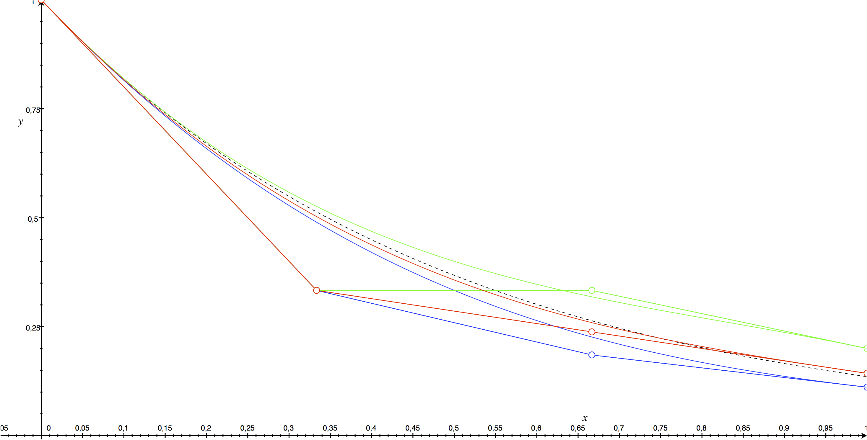
Even though \(\lambda \gg 1\) the curve stays close to the true solution (in dotted black). However in the (2,1) case we the see the appearance of an oscillation in the control points while the true exponential solution and all its derivatives are monotonic (The curve crosses its control polygon). The better accuracy of method \((2,2)\) is clearly visible.