Irreversibility, Conservation or Dissipation?
It was quite a revelation for me to understand that a dissipative LTI state-space system of the form
\[\begin{equation} \dot{\mathbf x}(t) = (J-R) \mathbf x(t) \end{equation}\]where \(J = -J^T\) is a skew-symmetric matrix that has an energy conservation role and \(R = R^T\) is a symmetric positive definite matrix that generates the Rayleigh dissipation rate \(\mathbf x^T R \mathbf x\), is equivalent to a nonlinear irreversibly modulated conservative Poisson system in higher dimension.
\[\begin{equation} \dot{\mathbf X} = J(\mathbf X) \mathbf X \end{equation}\]by extending the state vector \(\mathbf x\) with an entropy-like variable \(z\) that has the role of accumulating the dissipated energy.
To make it easier to understand let’s use a damped harmonic oscillator with the following dynamic equation
\[\begin{equation} \left[\begin{matrix} \dot x \\ \dot y\end{matrix}\right] = \left(\omega \left[\begin{matrix}0 & -1 \\ 1 & 0 \end{matrix}\right] - \sigma \left[\begin{matrix}1 & 0 \\ 0 & 0 \end{matrix}\right] \right)\left[\begin{matrix} x \\ y\end{matrix}\right] \end{equation}\]and the Hamiltonian energy function
\[H(x,y) = \frac{1}{2} (x^2 + y^2)\]It has pulsation \(\omega\) and dissipation rate \(\sigma\)
\[\begin{equation} \dot E(t) = \nabla H(\mathbf x)^T \dot {\mathbf x} = -\sigma x(t)^2 \end{equation}\]The equivalent in mechanics would be a mass-spring system with friction and in electronics a parallel RLC circuit.
Now let’s consider the augmented Hamiltonian.
\[H_e(x,y,z) = \frac{1}{2}(x^2 + y^2 + z^2)\]We wish to find the dynamic on \(z\) in order to have a conservative hamiltonian \(H_e(x,y,z) = C\), i.e. \(\frac{d}{dt} H_e(x,y,z) = 0\)
This is satisfied by the system
\[\begin{equation} \left[\begin{matrix} \dot x \\ \dot y \\ \dot z\end{matrix}\right] = \left[\begin{matrix}0 & -\omega & - \frac{\sigma x}{z} \\ \omega & 0 & 0 \\ \frac{\sigma x}{z} & 0 & 0 \end{matrix}\right] \left[\begin{matrix} x \\ y \\ z\end{matrix}\right] \end{equation}\]i.e.
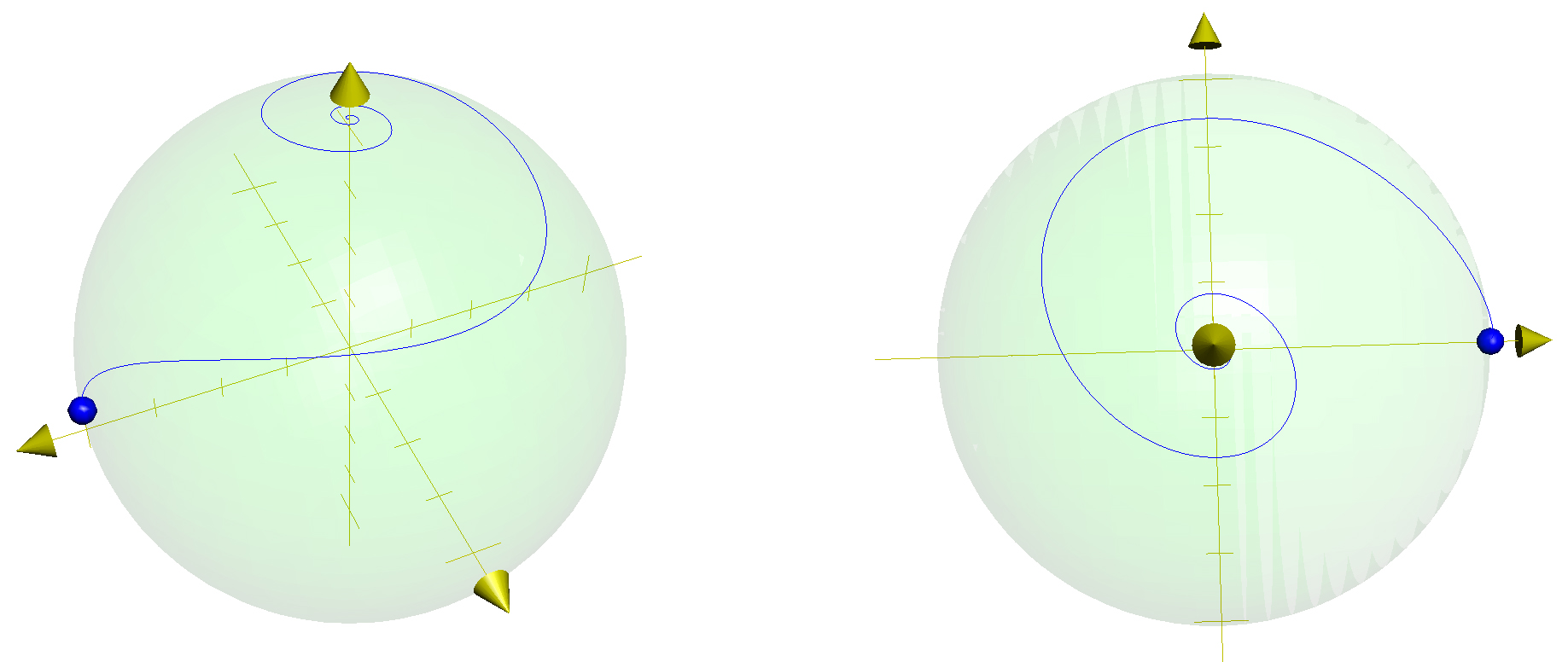
\[\begin{equation} \dot {\mathbf X} = J(\mathbf X) \mathbf X \end{equation}\]with \(J(\mathbf X) =-J(\mathbf X)^T\). We have converted a linear time-invariant dissipative problem to a nonlinear conservative time-variant one on the surface of a half-sphere (since \(z>0\)). Indeed its energy variation is given by:
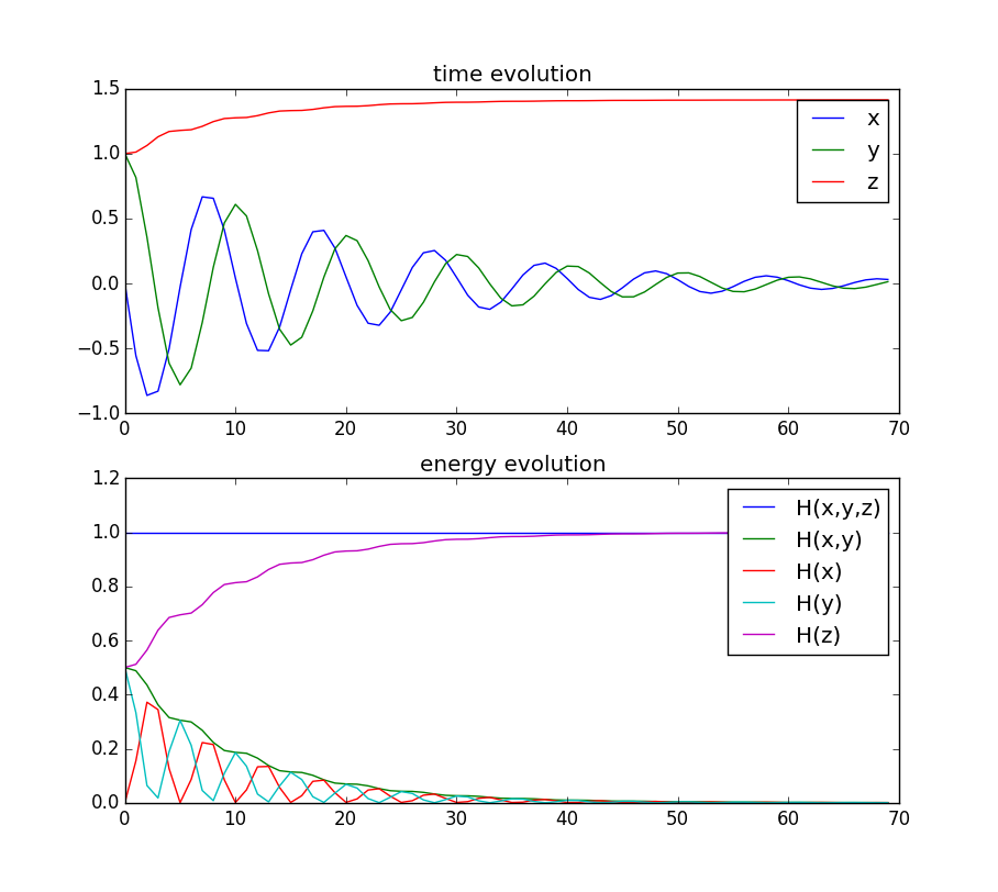
\[\begin{align} \dot E(t) = \nabla H_e(\mathbf X)^T \dot{\mathbf X} = -\sigma x(t)^2 + \sigma x(t)^2 = 0 \end{align}\]The consequence of this, is that any energy-preserving numerical scheme applied to the extended system has the side-effect of preserving the dissipative invariant.
The energy is indeed conserved and transmitted irreversibly toward the \(z\) coordinate.
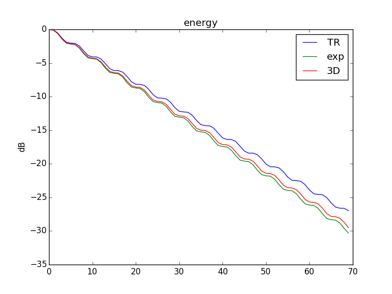
The decay rate is also closer to the exact solution with this approach compared to the Trapezoidal rule simulation
N.B.: in this example \(z\) is not an entropy, it is homogenous to the square root of an energy. Using an entropy instead would change the manifold from a sphere to a paraboloid. Because of the division by \(z\) its initial value shouldn’t be null and it raises the interresting question: “What was the initial value of the entropy of the universe”?
References:
- Daniel Fish. Dissipative perturbations of 3d hamiltonian systems, 506.
- Bernhard Maschke, Romeo Ortega, and Arjan J. van der Schaft. Energy-based lyapunov functions for forced hamiltonian systems with dissipation. IEEE transactions on automatic control, 45(8):1498–1502, 2000.
- P. J. Morrison. A paradigm for joined Hamiltonian and dissipative systems. Physica D Nonlinear Phenomena, 18:410–419, January 1986.