Rotary speaker modelling
While working on Rotary, I had to the time to perform extensive analysis of real rotary speakers. The usual ones like the Horn and Drum frequency and polar responses, the Doppler effect and some more unusual ones. Here’s some findings that I found interresting.
Angle-dependent delay
If we use several microphones around a moving acoustic source, by analysing the direct path propagation delay time from the source to each of the microphones, it is possible to infer the equivalent point-source trajectory as “seen” from the microphones.
In the case of a speaker rotating about a fixed center, if we setup 2 microphones at a 90° angle around the source, and plot the trajectory in the the \((D_L, D_R)\) plane, if the source was truely a point-source, we should see a circle trajectory because of the invariant \(D_L^2 + D_R^2 = R^2\) where \(D_L,D_R\) are respectively the distances of the speaker to the left and right microphones and \(R\) is the radius of the rotating speaker.
We did that and here’s the result we have for a rotary speaker horn
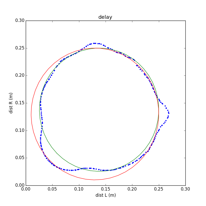
Indeed, we can see that we are not far from a circular trajectory but with an interresting side-lobes pattern. The horn is far from being a point-source and its static direct path propagation delay is angle-dependent because of the geometry of the Horn. These side-lobes have a noticeable impact on the Doppler effect which is not exactly sinusoidal and produces an more interresting frequency modulation pattern.
Doing the same kind of analysis on a rotating Drum speaker we see that we are getting further away from the circular trajectory.
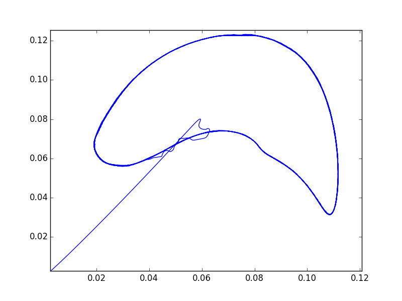
Indeed, the geometry of the Drum is closer to an open cube rotating about its axial center than to an ideal point-source.
Acceleration and decceleration curves
Another interresting aspect of these rotating speakers is that acceleration/deceleration curves are not symmetric because of the rotor inertia. Direct measurement was difficult to setup, so I decided to extract these from the signal amplitude and frequency modulation. My first attempt was using heterodyne demodulation and analysis similar to pitch-tracking to recover the rotating speed. However having very few information per revolution tn infer an acceleration curve makes the task quite difficult when the goal is to recover a continuouas acceleration curve. So I decided to move to a Bayesian estimation framework using Hidden Markov Models to add as much of a priori knowledge as I could.
Here is the raw speed observation probabilities I have after the feature analysis step:
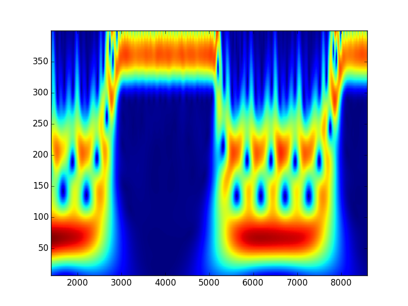
Quite ambiguous!
However, by adding a transition probablity model and using forward-backward decoding, the state probabilities are now much cleaner and easier to analyze.
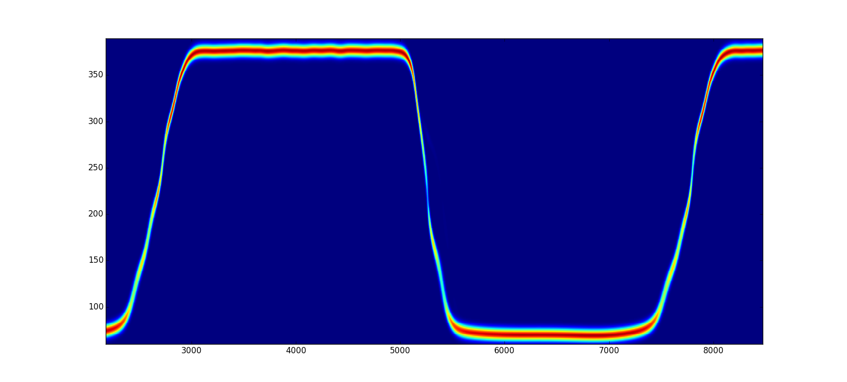
Image-source edge diffraction
Finally, if we decide to model the reflections within the speaker cabiner using the image-source method with a semi-open enclosure. And if we allow custom virtual microphone placement around the cabinet, we immediately have to solve 2 problems that don’t happen when the listener and the source are in the same room.
The first, which is quite common in ray-tracing is the visibility culling. Indeed according to the listener placement around the cabinet, the “visible” sources and the visibiity cone are changing according to the listener placement
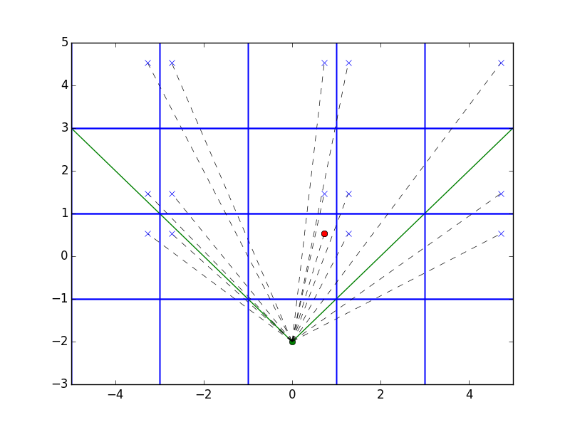
The listener is facing the open enclosure and quite close, its visibility cone is thus quite large, most image-sources are “visible”
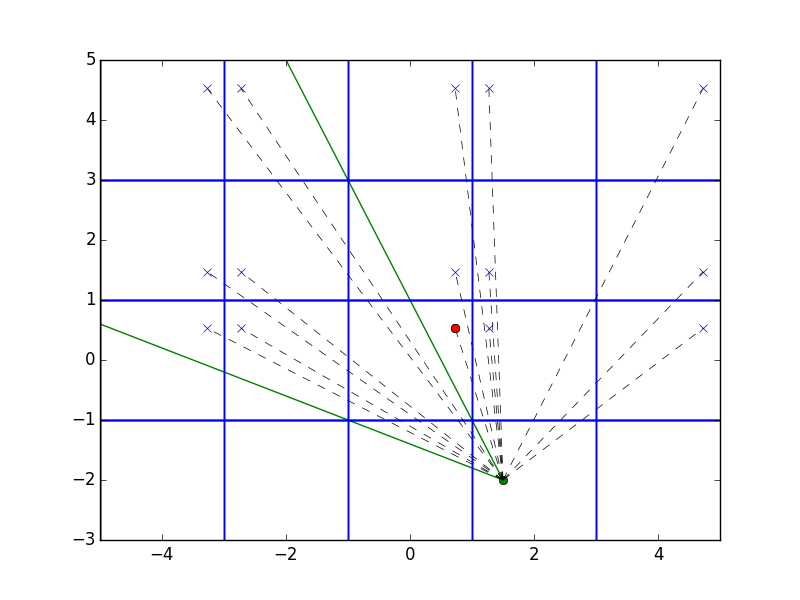
The listener is far from the open enclosure, its visibility cone is much smaller, many image-sources are “invisible”
Furthermore, since the source is rotating within the enclosure, according to the listener placement it can become alternativley visible and invisble within a revolution.
However, once we have solved this first problem, to continue the analogy with 3D ray-tracing, we immediately notice how problematic this kind of hard shadowing model can be. Indeed, sources appear then disappear discontinuously which in the audio world means annoying clicks and pops.
In the real world fortunately, thanks to the Huygen principle, things are much smoother. Any sound ray that encounter the edge of the enclosure, is diffracted in all directions as if the edge was an acoustic source.
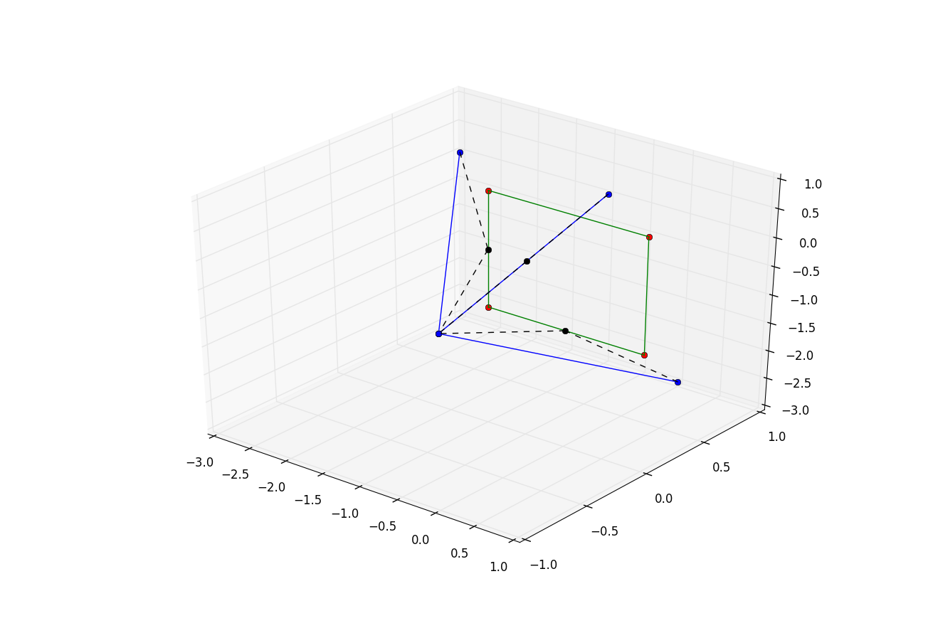
So even if a secondary source is “invisible” it still contributes to the acoustic sound-field measured by the microphones but with a different amplitude and propagation delay. Modelling this provides the soft-shadowing that was missing in the previous step.